Advanced Oscilloscope Triggering and Signal Isolation

How comfortable are you with advanced triggering on an oscilloscope? In my experience, having done training for thousands of professional engineers worldwide, about 90% of oscilloscope users know about only a fraction of the extensive list of advanced triggers offered to them in modern digital oscilloscopes. An autoscale and edge trigger may work well for basic measurements, but for debug and analysis of complex signals or physical layer glitches, advanced triggers can be an extremely powerful tool to help you get your job done faster. Today’s blog will focus on what exactly triggering is, and give you a basic primer on a great webcast that we’ve posted on our YouTube channel (see the link at the end of the article for more).

What is a trigger?

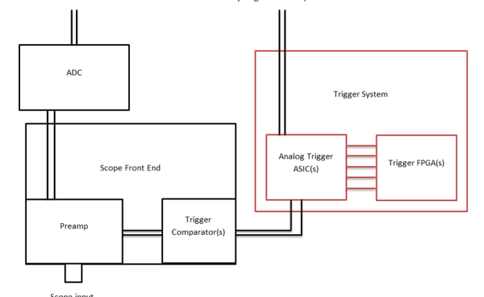
Most signals you are measuring are changing rapidly, thousands or millions of times per second. In order to take that rapidly moving data and present it to you in a coherent manner, an oscilloscope needs a trigger condition. As an example, let’s say I’m a photographer being hired by an equestrian to make a photo gallery of their horses for sale. Potential buyers, who will be viewing the photos, will want the photos to all have the same frame of reference so they can compare the sizes of each horse. If each horse’s photo is taken from different angle and distance, then comparing the photos to each other to see differences is basically impossible. But, if I take each photo from the left side at a distance of 5 meters, then the differences between the photos are clear so the buyer can make an informed decision of what horse they want.

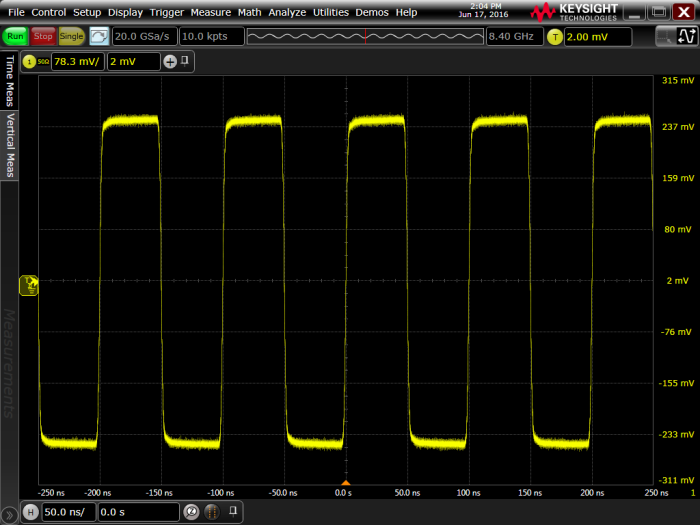
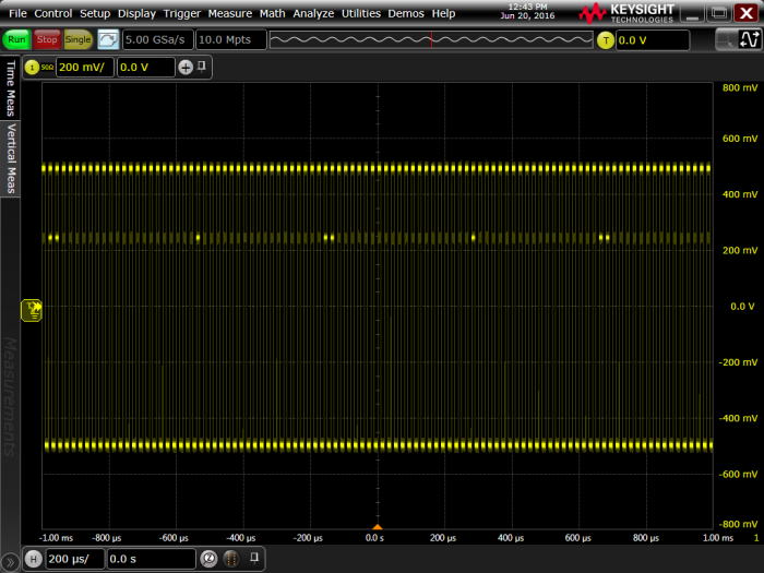
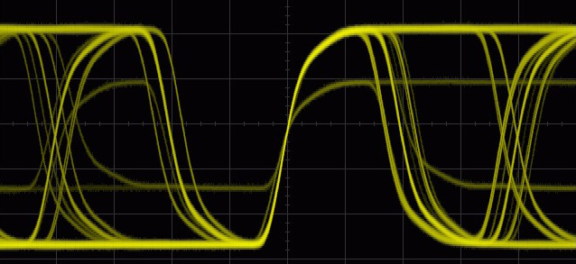
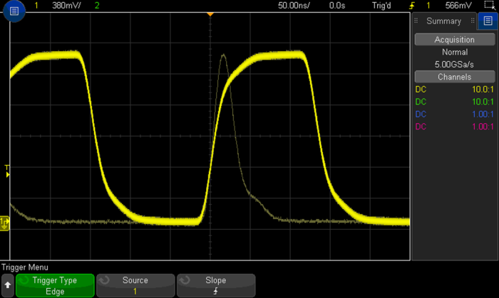
Oscilloscopes do the same thing. Today’s digital signals are complex. They are high frequency, non-repetitive, may have multiple logic levels, are often asynchronous, or are some kind of standardized serial protocol. The oscilloscope needs a rule for taking photos: when do you want a snapshot taken? The standard condition is an edge trigger. The oscilloscope takes a photo every time the signal crosses a defined voltage threshold. Consecutive photos are all overlaid on top of each other on the display, so you can view differences between each rising edge and look for anomalies. This can work well for something simple like a clock, but a complex multi-level signal may end up looking like this:

What if I am interested in one of these signals in particular? The rising edge trigger rule is not specific enough. That’s where advanced triggers come in: we need a more specifically defined rule to see exactly what we’re interested in!

Advanced Triggers

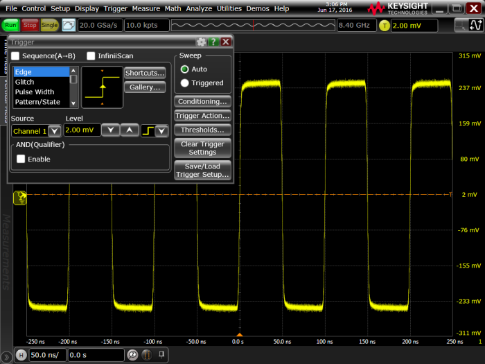
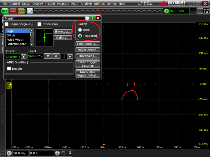
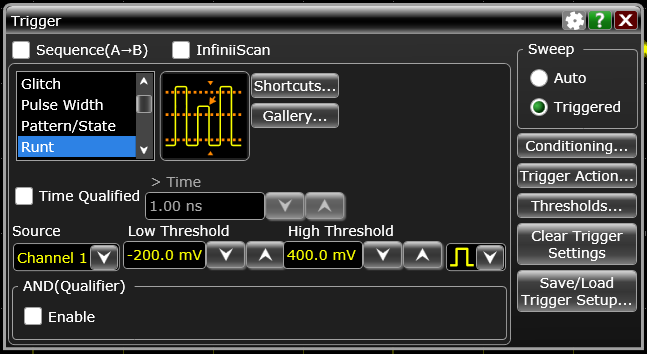
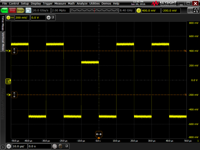
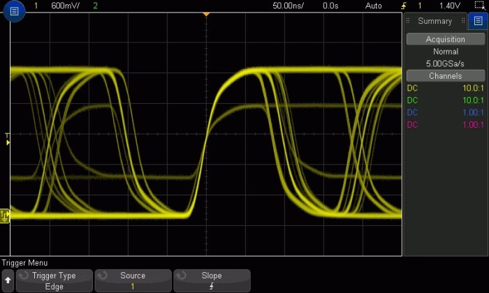
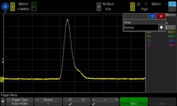
While the webcast goes over each trigger in detail, I’ll give an example of one here called pulse width trigger. With a pulse width trigger, we want the scope to take a photo if a signal rises and falls across a voltage threshold within a certain time restriction. In this signal, there is a clock with a pulse width of about 150 ns; you can see the signal crosses the trigger threshold in a rising direction, then again in a falling direction 150 ns later. The trigger threshold is visualized with the yellow T and arrow to the left of the screen, and timebase on top (50.00ns/division). But there is also a much smaller pulse the edge trigger is capturing, one that rises and falls again in under 50 ns:

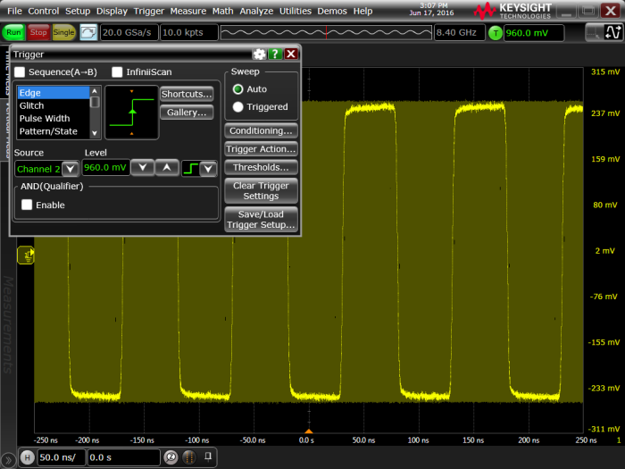
The basic edge trigger catches both. But by defining an advanced trigger, we can tell the scope to only take photos when the signal rises and falls across the trigger threshold in under 50 ns. Now, our picture is much more specific to what we want to troubleshoot:

Zone Triggering

Advanced triggers require some knowledge of the signal you’re testing, its shape and parametric qualities, as well as how to set the oscilloscope up properly. This is can be very difficult or nearly impossible for most scope users. Zone trigger was designed as a point and shoot system for isolating difficult signals within your design. This topic is covered in the webcast, or you can watch this video to learn more.

Serial Bus Triggers

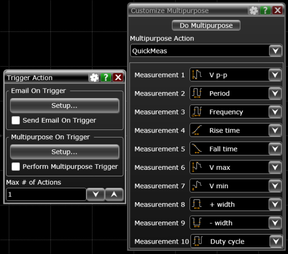
Keysight oscilloscopes also offer a suite of serial bus triggers. If you are working with an I2C bus and want to see when your device sends read commands to address 0x29, describing the shape of the signal as we did before simply will NOT work. We need a scope that is smart enough to translate the edge transitions in time to 1’s and 0’s and has knowledge of the I2C protocol. Here’s an example of the trigger capabilities for I2C:

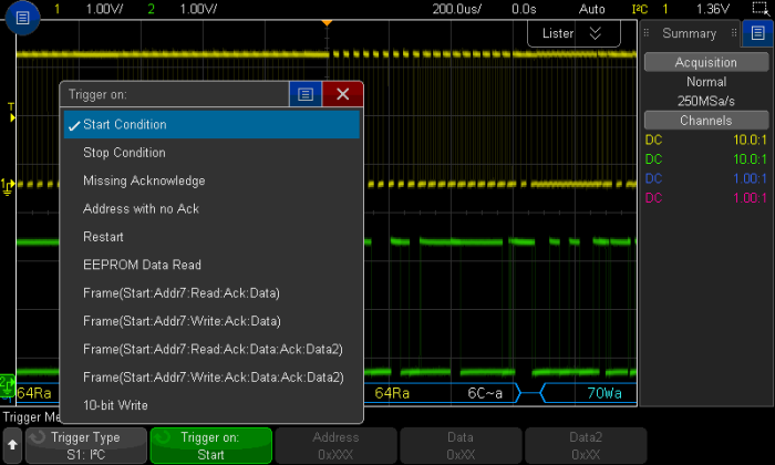
Read more about how oscilloscopes can decode serial data and find the product datasheets in this blog article.

Trigger Modes and Coupling

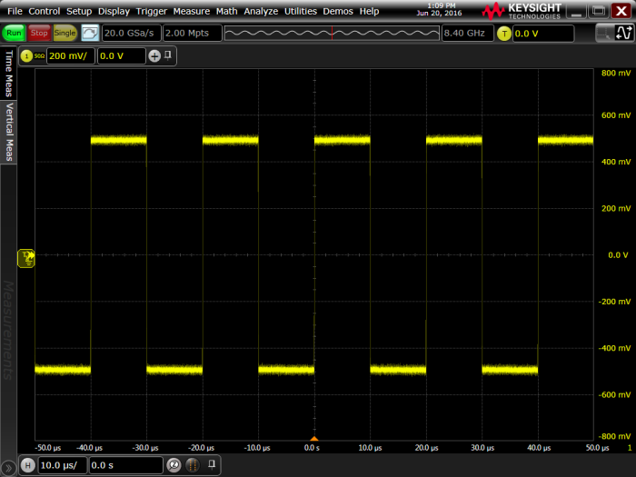
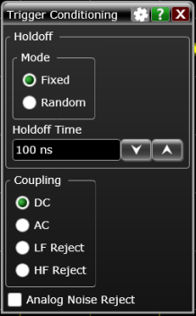
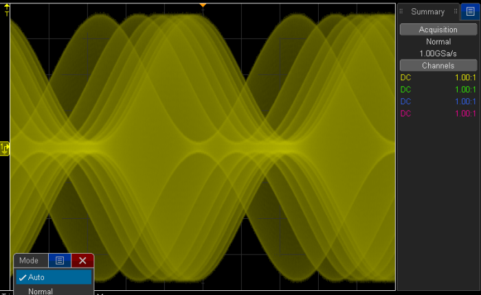
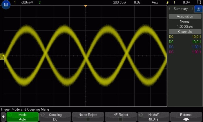
Life in the time domain is often a noisy one. And noise means triggering becomes difficult. For example, why is the scope triggering on rising and falling edges of the noisy signal below? If you zoom in, you’ll see that the falling edges of the sine wave contain small rising edges within it, that are large enough to qualify the oscilloscope to trigger. We cover all the different trigger modes and coupling techniques that can be used to make a more stable trigger in an unstable environment.  You might also try bandwidth limiting, as described aptly by Melissa here!

Summary

Advanced triggers can be difficult to master, and times when you need them are few and far between. Zone trigger can take a lot of that headache away, which is great. Mastery of the advanced triggers in oscilloscopes can not only separate the true power users from the rest, but also take your ability to solve problems in complex designs to a whole new level. Isolating a problem signal allows you to dive deeper in your debug process and fix bugs faster. Check out the recorded Advanced Triggering and Signal Isolation webcast on our YouTube channel.

Understanding Oscilloscope Trigger System Basics & Why You Should Care

You sit down at your lab bench to debug some funny behavior in a 10 MHz clock.  You fire up your oscilloscope, get your probing in place and hit the almighty Auto Scale button, after which you’re presented with something like this:

Figure 1: 10 MHz square wave after Auto Scale

and then it strikes you; there are ten million clock cycles occurring every second!  How in the world is the scope able to accurately display such a clean representation of your signal?  How is it that the middle of the rising edge of your clock is perfectly aligned at center screen?  The answer is the trigger system.

The trigger system is both one of the most commonly-used and least-understood sub-systems in real-time oscilloscopes.  In this article I’m going to pull back the curtain just a bit and explain what the trigger system does, how it works and why you should care.

 

What It Does

The sole responsibility of the trigger system is to tell the rest of the oscilloscope what data to care about.  It decides when the acquisition system begins acquiring, which means that by default it decides what is displayed on screen and what data is available to make measurements on.  It can make these decisions with a very simple set of conditions or very complex conditions, based on user input.  Let’s consider the example above; a 10 MHz square wave.  The reason the signal in the image above looks so clear and well-positioned on-screen is that the trigger is set up, appropriately, to look for a rising edge on Channel 1:

Figure 2: Trigger setup as configured by Auto Scale

Remember that to start we used Auto Scale, which was kind enough to pick an appropriate trigger source and threshold based on our input signal.  But what would our signal look like without an appropriate trigger configuration?  I’m glad you asked:

Figure 3: 10 MHz square wave, auto-triggered. Infinite-persistence is enabled on Channel 1 to better illustrate what’s going on

In Figure 3 above I have changed the trigger condition to look for an edge on Channel 2 (which has no signal connected at the moment).  The auto-trigger feature, which we can see is enabled in the “Sweep” section of the trigger configuration dialog, is automagically kicking off acquisitions on a regular time interval giving us a smear of yellow signal trace across the screen.  The signal itself appears to be clearly visible in this image, superimposed over the “smeared” signal trace, unfortunately however this is just an artifact of the screen shot; that’s where the signal happened to line up at the instant I took the screen capture.  In practice, auto-triggered acquisitions aren’t good for much of anything other than to determine the relevant DC parameters to use in setting up your trigger condition.  Note that if the auto-trigger feature is disabled, without an appropriate trigger configuration the oscilloscope simply won’t acquire:

Figure 4: Disabling the auto-trigger feature without an appropriate trigger configuration means the oscilloscope won’t acquire at all.

The trigger system will always place the trigger point (the instant at which all conditions present in the trigger configuration are met) at t = 0.0 s on screen.    Later on, we’ll see how using advanced trigger configurations can help capture infrequent and hard to find events, in addition to the simple rising-edge trigger we’ve seen so far.

 

How It Works

Most real-time oscilloscopes have an “analog” trigger system.  This system is actually a mishmash of analog circuitry and digital counters but it relies on input from analog comparators fed from the scope pre-amp.  Some oscilloscopes now feature a “digital” trigger, meaning that the trigger system is entirely digital and is fed with integer data from the ADC output.  Both types of systems perform the same function; evaluating whether or not all of the configured trigger conditions are met at a given moment in time.  Because fully digital trigger systems are fairly rare, we’ll focus on analog trigger systems.

Figure 5: Generic four-channel DSO front-ends and trigger system

Figure 5 above shows a generic representation of the parts of a four-channel DSO (digital-storage oscilloscope) that we’re concerned with; the analog channel front-ends and the trigger system.  The trigger system takes inputs from comparators on all of the analog channels and provides a single output.  For convenience, let’s focus on a simplified diagram with only one analog channel:

Figure 6: Generic DSO front-end and trigger system

Figure 6 is a simplified, one-channel view of the same systems depicted in Figure 5.  When a signal is connected to the channel input it goes through a series of transformations before it ends up on-screen:

• First, the signal is scaled appropriately and offset if necessary by the pre-amp. The pre-amp output is sent to the ADC to be digitized.

• Trigger comparators observe the output of the preamp and fire if it exceeds the threshold they have been set to. This threshold is set based on user input, or by helper routines like the almighty Auto Scale.

• The trigger system observes all of the trigger comparator outputs in the system and combines them in such a way as to monitor for a given set of conditions. These conditions can be very straight-forward (IE: rising-edge on channel one) or quite complex (IE: pulse-width greater-than 2.4 ns on channel 3, followed by a pattern of channel one high, channel two low and channel four low, held for a duration of greater-than 30.0 ns and less than 50.0 ns).

• When the trigger system sees that all of the conditions are met for the specified trigger, it sends a pulse on its output. We call this signal “System Trigger” or “SysTrig” for short.  SysTrig is monitored by the acquisition system as well as a special sub-system known as the “time-base interpolator”.

• When the acquisition system sees a pulse on SysTrig, it begins to digitize, process, store, measure and finally display data. We refer to this entire process in general as “acquisition”.

• Before the acquisition data (the waveform) which is now stored in memory can be displayed on-screen, we need to know how to orient it horizontally; this is where the time-base interpolator comes in. The interpolator monitors SysTrig, just like the acquisition system.  When it goes high, it’s the interpolator’s job to figure out what address in waveform memory matches up with the instant the trigger occurs.  It communicates this information to the acquisition system and voila, the result is the desired waveform on-screen, with the trigger point placed perfectly at t = 0.0 s!

 

Why You Should Care

Although some of you may find the inner workings of oscilloscope sub-systems interesting, it’s fair to say that most folks couldn’t care less.  If you are one of those folks and you just skipped the entire “How It Works” section above, no sweat, there will not be a quiz at the end!  The bottom line is that you should care about the trigger system and take the time to understand it because it can help you debug difficult issues and save you quite a bit of time and frustration.

Using an oscilloscope in a basic way, that is to say, pushing the Default Setup and Auto Scale buttons can tell us a little bit about our signal and is a quick and convenient way to get started.  However, if you’re interested in capturing an infrequent event, as is often the case when debugging common issues like runts, glitches and setup & hold violations, the trigger system is a powerful tool.

 

Advanced Trigger Modes

In addition to edge trigger mode discussed at the beginning of this article, most real-time oscilloscopes have a number of advanced trigger modes designed to detect common problems.  When used in conjunction with “Triggered” sweep (aka, auto-trigger disabled) these modes will ensure that only the behavior you’re looking for is acquired and displayed.  As an example, let’s look for a runt in a square wave.  We connect our signal, use our trusty Auto Scale button and all we see is a square wave, no runt in sight!

Figure 7: Looking for runts in all the wrong places…

Figure 7 shows us that although we suspect a runt is present in our signal, finding it with edge trigger will prove difficult.  Maybe we’ll be able to see it if we zoom out a bit?

Figure 8: Looking for a runt with edge trigger, zoomed out horizontally

As shown in Figure 8, by zooming out horizontally we can tell that there’s something fishy going on, but it’s not entirely clear what.  Now, let’s use runt trigger mode on our Infiniium S-Series oscilloscope and see what we can find:

Figure 9: Runt trigger mode setup on an Infiniium S-Series oscilloscope

 

Figure 10: Looking for a runt with runt trigger mode

There’s our runt!  The waveform in Figure 10 is clear and steady and the event we’re interested in, our elusive runt, is right at t = 0.0 s!  This is the value of learning the trigger system on your scope, it will allow you to find the events you’re interested in, and only the events you’re interested in, very quickly.  Although this example focused on finding a runt, the same sort of example can be demonstrated with glitches, setup & hold violations, specific data across multiple channels, data patterns relative to clock edges, edge transition times, etc. using the appropriate trigger mode.

 

Advanced Trigger Features

In addition to advanced trigger modes like runt mode discussed above, many oscilloscopes have features that can be used in conjunction with trigger modes to further refine what we want the oscilloscope to show and to instruct the scope to automatically take actions when a trigger occurs.

Figure 11: Trigger Conditioning dialog on an Infiniium S-Series oscilloscope

Figure 12: Trigger Actions available on an Infiniium S-Series oscilloscope

Figure 11 above shows some common options for trigger conditioning, while Figure 12 shows some of the things we can configure the oscilloscope to do for us automagically when a trigger occurs.  My personal favorite is the “Email on Trigger” feature.  If you have a really infrequent event, no problem; set up your trigger and leave for the weekend.  Come back, open up your email and find all the data you need!

Thanks for reading!  If you have specific questions regarding triggering or challenges triggering on a specific event let us know in the comments!

Oscilloscope Triggering: When is Normal not so Normal?

Oscilloscopes have two primary modes of triggering: AUTO and NORMAL. However, NORMAL is not the normally used mode of triggering. AUTO is. The default trigger mode in all of today’s oscilloscopes is AUTO. There is a lot of confusion these days among oscilloscope users as to exactly when to use which mode of triggering. Let’s first define what these terms mean and then discuss how these modes of triggering came to be called what they are.

AUTO simply means “automatic”. In the AUTO trigger mode, the scope will trigger on the signal under test if a trigger condition is met, such as a rising edge. But if a trigger condition doesn’t occur within a predetermined amount of time, the scope will begin to generate its own automatic triggers, which are not synchronous to the signal under test. This means that the scope will show of blur of waveforms when this happens. So if AUTO is always the default trigger mode, why would you ever want to see a blur of waveforms? One reason is that a blur of waveforms will show you where the signal is relative to your trigger level. Perhaps you have the trigger level set above (too high) or below (too low) the signal under test. With AUTO trigger you can see what’s wrong and make adjustments. Setting up an oscilloscope is an iterative process of seeing what’s there and then making adjustments (V/div, sec/div, trigger level, etc.) until it is right. Another reason the AUTO trigger mode is the default mode of triggering is that you may want to simply view the DC level of a power supply. Scopes can’t trigger on DC, unless the DC includes lots of switching noise, in which case it is not purely DC.

The NORMAL trigger mode means that the scope triggers if and only if a trigger condition is met. If you’ve got your trigger level set above or below the signal under test, then you’ll be looking at a blank screen on your scope. So when should you use NORMAL triggering? If the signal you want to trigger on occurs very infrequently, perhaps once every three seconds, then you should use the NORMAL trigger mode so that the scope will display synchronized representations (waveforms) of your signal only when trigger event occurs, and not generate automatic and asynchronous triggers between qualified trigger events and thereby show you blurs of waveforms.

So why is this trigger mode call NORMAL? I can only guess. Back in the old analog scope days, this trigger mode was not called NORMAL triggering. It was call the TRIGGERED sweep mode, which makes sense. When a trigger qualification was met, such as a rising edge, the analog scope would trigger a linear sweep of an electron beam across the scope’s cathode ray tube (CRT). But when digital storage oscilloscopes (DSOs) came along about 30 years ago, the representation of waveforms on the scope’s display changed from the sweep of an electron beam that excites phosphor on the CRT to the digitization and storage of discreet waveform points using an analog-to-digital converter (ADC) and then represented as pixels on a scope’s display. Since newer technology scopes stopped sweeping, most oscilloscope vendors began calling it a “trigger” mode instead of a “sweep” mode. And if they had kept using the same old analog scope terminology it would have become the TRIGGERED trigger mode, which sounds redundant. So some genius marketing guy must have said, “Let’s call it the NORMAL trigger mode — maybe because it was the trigger mode that he or she normally used.

Note that some DSOs still call it an AUTO and TRIGGERED sweep mode. I feel sorry for the younger engineers that have no idea what a sweep is.

In my opinion the AUTO and NORMAL trigger modes should be called AUTO On/Off. To me, this makes more sense. But I know that’s not going to happen, just like Australians will never stop calling their oscilloscopes their “crows”, which I think will be the topic for my next blog.

Anyone out there know for sure how this mode of triggering came to be called NORMAL?