How to measure your oscilloscope (and probe)’s bandwidth yourself

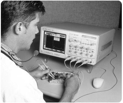
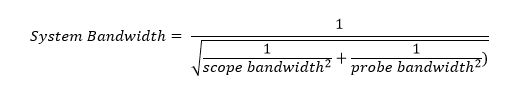
Customer visits are not only exciting, but excellent learning experiences.   My visits with customers cover a range of topics from answering questions on specific technical capabilities to presenting the latest technologies to researching product use models.  In these visits, I often demonstrate product features and benefits when using oscilloscopes. However, it is also common that customers show me their oscilloscope measurement tips that blow my mind.  My first blog talked about the formula to figure out system bandwidth (the bandwidth of the scope + the probe). Now let me share a neat measurement where you can quickly find the “true” bandwidth (or system bandwidth) of your oscilloscope yourself, a tip that a customer taught me about 15 years ago.

“Let me test it to see if your new scope REALLY has 6 GHz bandwidth” said a customer in the very first VIP visit disclosing Keysight’s (then Agilent) first 6 GHz real-time oscilloscope.  This caught me by surprise as no previous customers I had ever met had made such a statement.

“I need to connect my fastest step response generator to your scope’s front end first”.  He plugged in his faster-than-50-ps edge rate step signal generator and then differentiated the signal using the “differentiate” math function to derive the impulse response signal.  He continued and applied the “FFT” (Fast Fourier Transform) math function to the calculated impulse response signal in order to plot the frequency content from DC all the way up to 6 GHz (and beyond).  Finally, he nodded, smiled and told me, “Excellent and congratulations!  Your scope has more than 6 GHz of analog bandwidth” by pointing out the FFT plot where the FFT value finally attenuated down by -3 dB (the bandwidth point).

In theory, a perfect step response has an instantaneous (zero) rise time, and therefore you can mathematically derive the perfect impulse response by differentiating it.  And in theory, the perfect impulse response signal has an infinite amount of frequency content, so it is a perfect signal to check the “finite” bandwidth limit of an oscilloscope’s front end.  No signals are perfect, but the fast edge rate step generator can serve this purpose well.  Wow, what a quick and clever way to test the system!  Ever since this customer visit, this has become my favorite method to demonstrate an oscilloscope’s front end bandwidth performance.

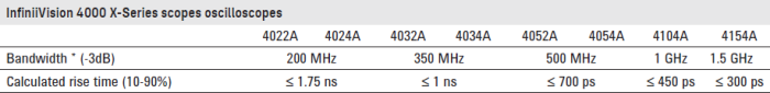
Alright, enough of a nostalgic story. Here are the step by step instructions with oscilloscope screenshots for you to duplicate this “measure of your oscilloscope’s true bandwidth” procedure.  As I wrote in my first blog, most oscilloscopes come with a little “more” bandwidth than what’s specified in their datasheet, so this may be a fun exercise!  The procedure will be a little simpler if you have a Keysight InfiniiVision X-Series (3000A/TX, 4000X or 6000X) oscilloscope because you can generate a pretty fast step response using the trigger out function of the X-Series.  You can alternatively use your favorite step generator, but be sure the edge rate is fast enough to contain enough frequency to test your oscilloscope.  I recommend using an edge rate more than twice as fast as the calculated rise time specified in the scope’s datasheet.  Also, note that the accuracy of your measurement heavily depends on the cleanness/flatness (signal integrity) of the input step response.

InfiniiVision Series Oscilloscopes	Trigger out edge rate
6000 X-Series (DSO/MSO-X 6000A)	~ 700 ps
4000 X-Series (DSO/MSO-X 4000A)	~ 1.4 ns
3000 X-Series (DSO/MSO-X 3000A/T)	~ 1.7 ns

Table 1:  The summary of the trigger out signal’s edge rate

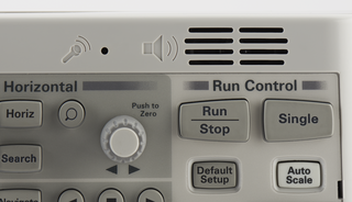
 Step 1: Connect a fast edge rate step response signal.  The below example uses the trigger out signal of the InfiniiVision 6000X (~700 ps edge rate).  Scale the signal so the edge gets placed at the center of the screen.  Make sure to vertically maximize the signal without clipping it in order to use full 8 bit resolution of your scope’s analog to digital converter (see the blog post “This Quick Trick Makes Your Oscilloscope Measurement 1,000 Times Better” for more detail).  Change the channel’s input impedance to 50 Ω to match your source.  Usually, a fast step generator has an output impedance of 50 Ω.  The output impedance of the InfiniiVision X-Series oscilloscope’s trigger out signal is also 50 Ω.

Step 2:  Apply the differentiate math function to your step response signal (channel 1 in this example).  For the Keysight InfiniiVision oscilloscopes, the differentiate math function is available on the 3000AX, 3000TX, 4000X and 6000X.

Figure 1: The step response signal (yellow) and the math function impulse response signal (purple)

Step 3: Apply the FFT math function to your impulse response signal (math function 1 in this example).  For the Keysight InfiniiVision oscilloscopes, the FFT math function is available on all models.

Figure 2: The step response signal (yellow) and the math function FFT plot (purple) of the impulse response signal

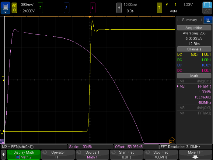
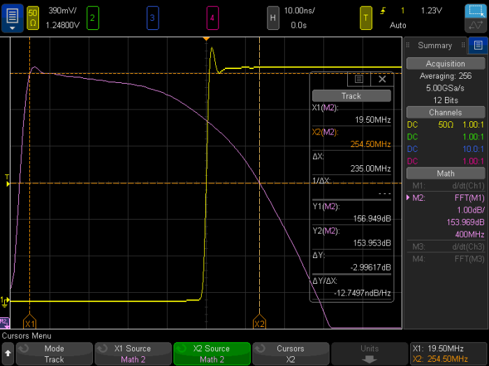
Step 4:  Turn on cursors to measure the frequency where the signal is attenuated by -3 dBm.  You can read the ΔY value in the cursor readout to precisely determine this point.  This is the “true” measured bandwidth of your oscilloscope.  In this example, it measured the “true” bandwidth of a 200 MHz InfiniiVision MSO-X 4024A to be around 250 MHz while the product’s specification says 200 MHz.  A nice bonus of an extra 50 MHz.

Figure 3: Measuring the oscilloscope’s bandwidth using the cursor

Now, let’s expand the same concept to measure the system bandwidth of your oscilloscope and probe. A similar connection can be used, however, it will require a probing point for the probe to pick up the signal.  What I usually use is a 50 Ω microstrip line fixture like the ones shown below.

Figure 4a: Handmade microstrip line 50 ohm fixture

Figure 4b: Keysight E2655C Probe deskew and performance verification kit

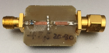
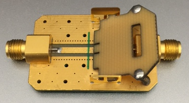
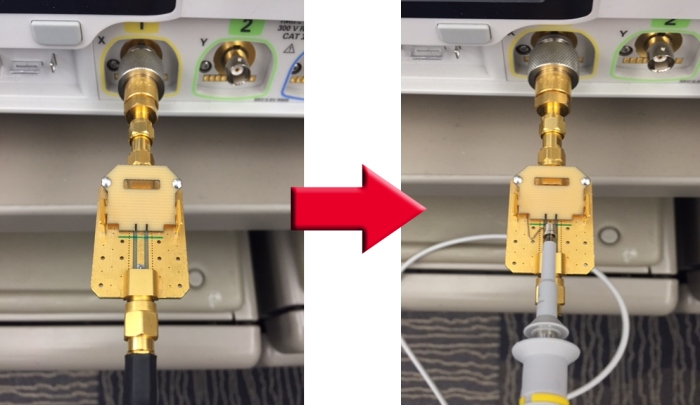
Insert the fixture between the cable and the scope’s BNC channel input and then probe the signal with the probe you want to measure the system bandwidth for.

Figure 5: Connecting the probe to the fixture

Once you have the probed signal on screen, just repeat the steps describe above.  The next section shows two screenshots from the system bandwidth measurements done on the 200 MHz scope; 200 MHz scope + 100 MHz passive probe and 200 MHz scope + 200 MHz passive probe.  You will note the “true” bandwidth is higher than the calculated bandwidth, since both oscilloscope and probe usually have a slightly more bandwidth than they specify.

Figure 6: 200 MHz oscilloscope + 100 MHz probe system bandwidth

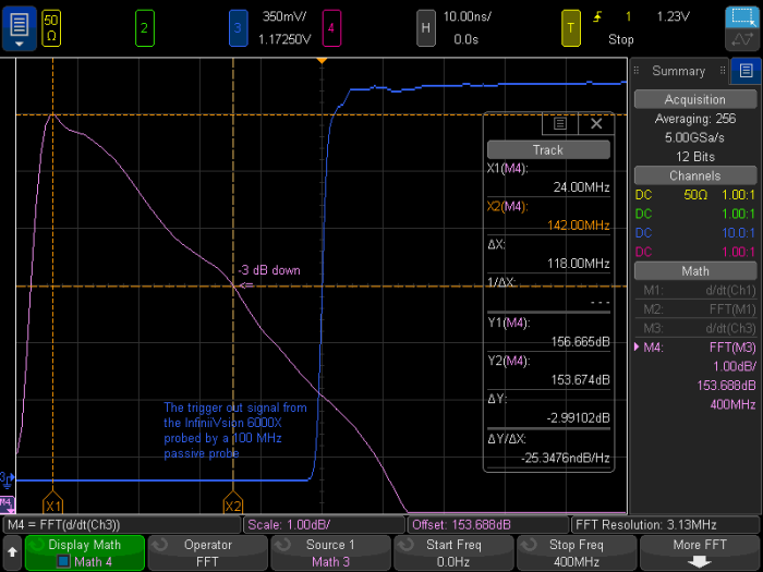
For example, the measured system bandwidth in Figure 6 is around 140 MHz.  If you were to use the formula from the previous blog, the theoretical system bandwidth of a 200 MHz and a 100 MHz probe should be around 90 MHz, so you are getting ~ 50 MHz more due to “bonus” bandwidths on the scope and the probe.  In fact, because you already know the true bandwidth of this 200 MHz scope is around 250 MHz, you can easily find that this 100 MHz passive probe actually has around 170 MHz bandwidth using the same formula!  Note, I’m assuming both the scope and probe have the Gaussian response filter.

Figure 7: 200 MHz oscilloscope + 200 MHz probe system bandwidth

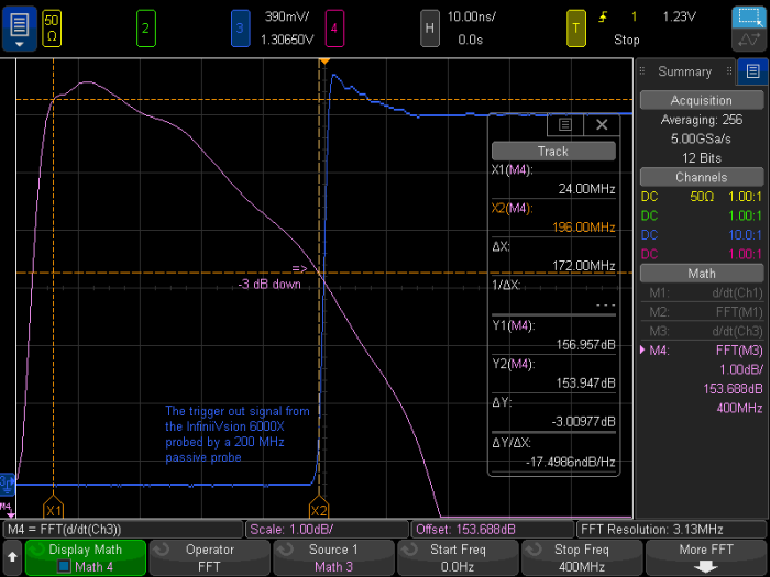
In the final example, it measured system bandwidth to be around 200 MHz, as seen in Figure 7.  Applying the same formula, you can calculate quickly that this 200 MHz probe actually has more than 300 MHz bandwidth, 100 MHz additional bandwidth beyond the specified value!!

“Hello Scope” – Oscilloscopes Past and Present

I bought my first car navigation system, or “nav”, back in 2000. I believe I was still one of the “early adopters”; however, the car nav was already becoming a popular car electronic in Japan by then.  Actually, it was a pretty fancy one with a retractable display, 3D virtual map, built in gyro-compass (so it would still provide guidance even when satellite signals were lost), altitude meter and more.  However, what impressed me the most was the “full voice control system”.  “Take me home”, “call my mom”, “100 m scale”, “avoid traffic jam” were some of the popular commands I used back then.  Oh, yeah, and the nav even spoke different Japanese dialects depending on the location and setting I chose.

Coincidently, year 2000 is when I joined Keysight, (Agilent at the time). Joining one of the most technically savvy companies in the industry as an oscilloscope product line manager, I had a high hope of “what if oscilloscopes can hear my voice, too”.

Well, Agilent (Keysight) certainly did not disappoint me. In fact, did you know that Agilent has had a voice control enabled oscilloscope since 1999?  The product was called “Option 200: VoiceControl for Agilent Infiniium Oscilloscopes (E2635A)”.  Here is the picture from the original datasheet.

The option understood popular scope operating commands like “Run”, Stop”, “Default Setup” and “Auto Scale”. It controlled the vertical setting (like volts/div), horizontal controls (like time/div or delay sweep), and trigger and storage commands.  In another words, the most popular operations were possible via voice commands… in 1999!  In fact, many of my customers back then were asking for a scope “foot switch” for those operating it hands-free in the manufacturing line or engineers holding two probes in both their hands.  “Wow, this must be a perfect solution, just like I loved my car nav voice commands!”  At least, this was my first reaction as a first year product line manager.  Well, it did not come out to be exactly that way.

First it understood English, to be specific American English, but nothing else. Growing up in the US, I had no problem using it. Believe it or not, it didn’t understand my good-old colleague’s British English!  Obviously it did not understand Japanese and perhaps had a lot of trouble with “Asian pronounced English” as well.  There was no “Siri” back then and I guess I don’t need to talk about the sales results.  However, I thought it was a brilliant idea as the fundamental needs were there.  Second, as you can see on the image above, one must use an included special “microphone” when talking to the scope, which was just one more device to lose.

Now, let me fast forward the clock to the year 2014, 15 years after a great but crazy innovation. If my memory is correct, no other oscilloscope vendors released another voice control enabled scope since the Infiniium option 200. And so Keysight tries again, in the era where voice control is a lot more pervasive, again thanks to Siri and Google devices in the market.

So, the new InfiniiVision 6000 X-Series oscilloscopes released in April 2014 comes with the world’s only voice control system, but this time with 14 different languages and dialects, including English (American), English (British) and English (Indian)! And yes, it understands Japanese as well.  Furthermore, no dorky microphone is needed this time.  And off course, now it is powered by the Nuance Communications, Inc. voice recognition engine (the company who build the Siri voice recognition system).

 

So, the next time, you see the InfiniiVision 6000 X-Series scope, make sure to say “Hello Scope” and it will gladly listen and respond to your commands in most languages around the world.

What’s the next crazy and innovative idea? What should all scopes have as a standard feature in 2030, another 15 years from now?  As a Keysight oscilloscope planner, my job is to help realize your craziest oscilloscope dreams!  Let me know!!

What is oscilloscope system bandwidth and how do I find the bandwidth of the scope + probe?

“I am using a 100 MHz oscilloscope with an included 100 MHz passive probe, I am supposed to be able to measure a 90 MHz sine wave, right?  Is the scope or probe broken?”

I hear this sort of question popping up from time to time, understandably since most oscilloscope datasheets do not discuss the “system bandwidth” or your effective bandwidth when a scope is used with a specific probe.

Both an oscilloscope and a probe have bandwidth specifications, the frequency value where the amplitude of input signal attenuates by 3 dB.  So, if your scope’s datasheet specifies its bandwidth at “100 MHz”, you are guaranteed to measure at least ~70% of your signal amplitude at its bandwidth frequency.  The same can be said for your probe as well.  The tricky part is, however, your oscilloscope + probe bandwidth, or your “system bandwidth”, may not be 100 MHz when you use them together. So, what is the system bandwidth in this case?

Before knowing your system bandwidth, you need to know the front end filter response of your oscilloscope.  You may or may not find this info in the datasheet, so call your scope’s support line if it is not stated.  If you don’t want to call/write the support line, I’ll provide you a quick tip to figure this out by just looking at the calculated rise time specifications in datasheets at the end of this blog.  However, it is a good rule of thumb to think the filter is a “Gaussian” type if the bandwidth of your scope is below 1 GHz.  For oscilloscopes with 1 GHz or more bandwidth, it could have a filter type called a “Brickwall”.

In the case of the Gaussian filter, which is the traditional front end filter type used for decades in both analog and digital storage oscilloscopes, the scope and probe’s system bandwidth is calculated using the below formula.

Let’s apply the above example to this formula.  Since your scope’s and probe’s bandwidth are 100 MHz each, your system bandwidth will be 70.7 MHz.  In other words, your signal’s amplitude is attenuated by 3 dB at 70.7 MHz.  Obviously, you will not see full amplitude of a 90 MHz sine wave!

In reality, most of oscilloscope manufacturers add some margin to the bandwidth specifications of both scopes and probes.  So, if you see the specification says “100 MHz”, it most likely has some additional bandwidth, like 110 or 120 MHz.

Now, say if you have a “Brickwall (or maximum flatness)” type filter response oscilloscope and probe instead.  It is extremely rare to see the Brickwall filter on a 100 MHz scope, but for this example say you did.  In such case, unfortunately, the former “square root of sum of squares” formula cannot be used.  In this case, the system bandwidth formula will be:

System Bandwidth = min {scope bandwidth, probe bandwidth}

So, if I apply the original example to this formula, your system bandwidth is now at 100 MHz, therefore, you should see nearly full amplitude of your 90 MHz sine wave.

I am not sure why this simple formula has disappeared from most oscilloscopes’ datasheets.  Perhaps there is more than sufficient bandwidth in most oscilloscopes today where engineers do not need to operate them at their upper limits.  Perhaps this is already taught in school.  Nevertheless, this is a quite useful tip to know, especially if you are seeing unexpected measurement results.

BTW, here is a quick and dirty way to determine if your scope has the “Gaussian” or “Brickwall” type response filter.  First, find your scope’s calculated rise time info.  The below is an example from Keysight InfiniiVision 4000X oscilloscope.

Now, divide “0.35” the calculated rise time value.  In the case of the 200 MHz oscilloscope (4022A), it will be

0.35 / 1.75 ns = 200 MHz

So, you verified the coefficient it was used to calculate the rise time was “0.35”.  0.35 is the coefficient value for a “Gaussian” response filter, so you know this 200 MHz oscilloscope has a Gaussian filter front end.  On the other hand, if you apply the same formula to 1 GHz oscilloscope (4104A),

0.35 / 450 ps = 778 MHz

The value was 778 MHz and not 1 GHz.  Well, you now know the coefficient used for this oscilloscope was not “0.35”, but was “0.45” (0.45 / 450 ps = 1 GHz).  When the coefficient value is larger than 0.35 such as 0.4, 0.45 or even 0.5, it indicates the scope’s front end has a filter response closer to the Brickwall filter.

Hope this small tip helps you to understand the scopes better.  See you all in the next blog!