How to extend SNR in wideband oscilloscope-based pulsed RF measurements

Keysight Oscilloscopes Blog is moving! Come check out the same great content in our new location: https://community.keysight.com/community/keysight-blogs/oscilloscopes.

In urban slang, signal-to-noise ratio (SNR) is a simple enough concept: the ratio of useful to useless information. We all know people whose SNR is not as high as we might hope. Unfortunately there’s no technology yet available to boost their SNR.

So engineers can be happy that’s not true for RF signals. We can now extend SNR in wideband oscilloscope-based RF measurements through what’s known as “processing gain.” Digital down-conversion lets you see small pulsed RF signals next to large signals by reducing the noise level in a particular measurement—whether it’s RF pulse envelope characteristics or frequency or phase shift across a pulse.

Increase in pulsed RF capture dynamic range

So how does it work? The trick is adding vector signal analysis (VSA) software. VSA in conjunction with an oscilloscope can extend the SNR. First VSA shifts a captured signal down to baseband I/Q. Then it bandpass filters the acquired oscilloscope data and finally resamples the data at a lower sample rate. The result is lower noise, higher dynamic range, and a wider SNR.

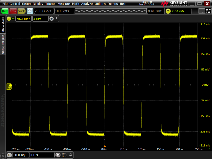
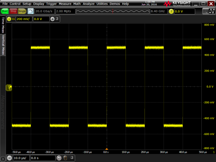
Let’s look at an example: An 8 GHz-wideband oscilloscope captures a pulse train in which a large pulse is immediately followed by a small pulse that is 50 dB down from the first pulse. This corresponds to being 100,000 times lower in power and ~316 times smaller in voltage (sqrt[100,000]) than the first pulse. The two-pulse sequence then repeats.

The large pulse has a +6 dBm power level (~1.4 mW), which results in a peak voltage of around 633 mV into 50 ohms. This can be represented as a -4 dBVpk level (20log 0.633). It also corresponds to a 1266 mV peak-to-peak signal into 50 ohms.

In contrast, the small pulse, being 316 times smaller in voltage, is only 4 mV peak to peak (-44 dBm, -54 dBVpk).

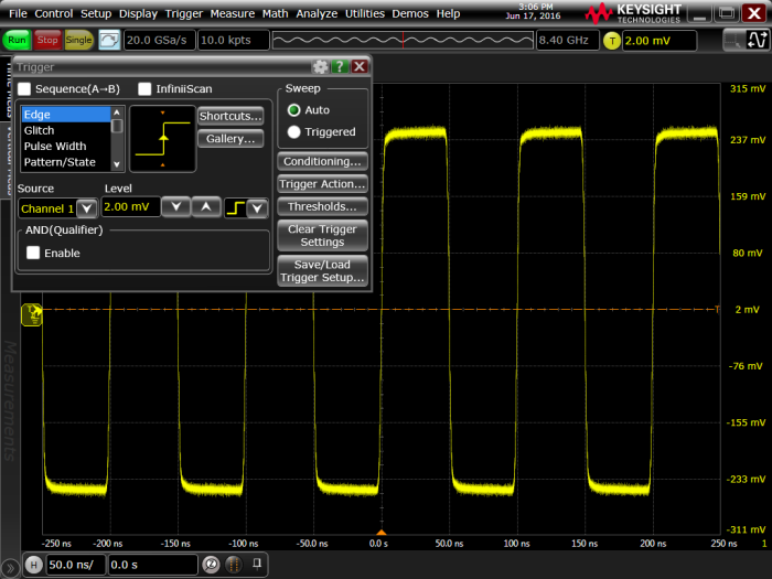
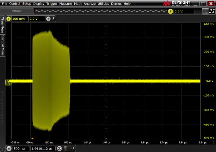
The VSA software, which also controls the oscilloscope front-end sensitivity, is set to +6 dBm (633 mV peak). This corresponds to an oscilloscope vertical range of 1266 mV.  There are eight vertical divisions, so this also corresponds to a ~160 mV/div setting.

At the full 8-Hz bandwidth for this ~160 mV/div setting, the broadband RMS noise for the 8 GHz bandwidth oscilloscope is around 5 mV, interpolating from a noise chart in the data sheet, as shown in Table 1.  The 5 mV of noise translates roughly into a peak-to-peak noise that is three times the RMS noise (assuming Gaussian noise). In other words, we’re looking at 15 mV of peak-to-peak noise.

Table 1. 8-GHz bandwidth oscilloscope RMS noise levels at various V/div settings

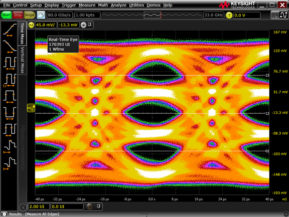
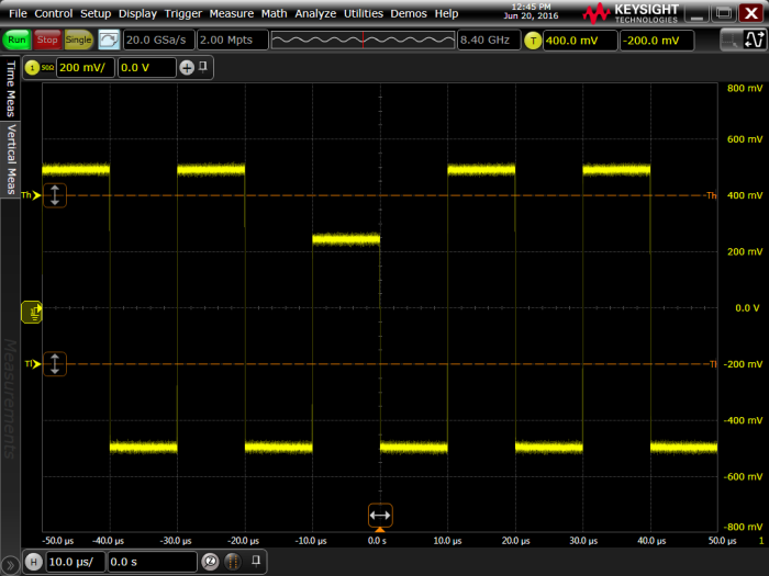
The small pulse (4 mV p-p) is masked by the noise in the measurement (15 mV p-p). (Think how easily a big-mouth can drown out softer-spoken colleagues.) The small pulse can’t be well-discerned in the full 8-GHz measurement of the oscilloscope, with a linear scale and no averaging, as shown in Figure 1.

Figure 1. 8-GHz bandwidth oscilloscope capture of +6 dBm pulse next to a 50 dB down pulse (2nd pulse cannot be seen)

 

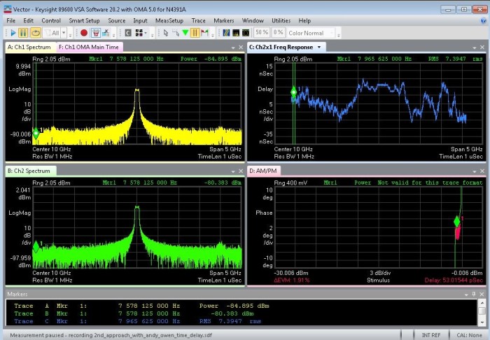
Import of real-time captured pulsed RF signals into analysis software and digital down-conversion

Basic pulsed RF measurements can be made natively on a high-bandwidth oscilloscope. And there are certainly times that measurements on directly sampled signals are desired. But this isn’t one of those times. Instead we’re looking for advantages available through external signal processing and analysis on captured signals.  For example, through a process called digital down-conversion, it’s possible to make a range of RF pulse measurements with higher accuracy. That’s due to the lower noise present by using processing gain. Let’s take a closer look.

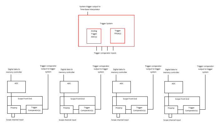
Figure 2 shows the basic process of digital down-conversion.  Through digital signal processing, the oscilloscope samples are multiplied by the sine and cosine of an imaginary oscillator of frequency f_c, where f_c is generally chosen to be the center frequency of the signal of interest. In effect, we’re “tuning” to the frequency of the input signal. This process converts the time samples into real and imaginary number pairs that completely describe the behavior of the input signal. To reduce noise, these samples can be low-pass filtered and then re-sampled at a lower rate to reduce the size of the data set and allow FFT processing of the data at a later stage. The resulting digitally down-converted samples can then be placed into memory for further processing.

Figure 2. Oscilloscope-captured samples input to VSA software for digital down-conversion

 

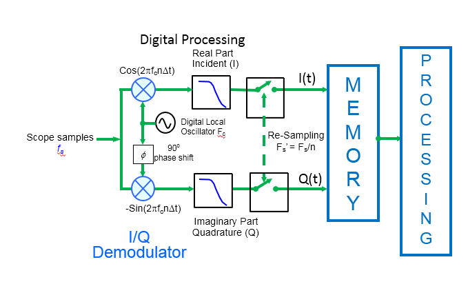
Some important demodulation information comes from this digital down-conversion process. First, consider what happens when the digital local oscillator frequency F_c is equal to the carrier frequency of a modulated signal. The output of the digital filters, which includes the real part I(t) and imaginary part Q(t), consists of time-domain waveforms that represent the modulation on the carrier signal.

Do you want that in math? Here’s a representation of the captured input signal:

=  A(t) * Cos[2pf_ct +q(t)]

where the following equation describes the amplitude modulation:

And the equation here describes the phase modulation:

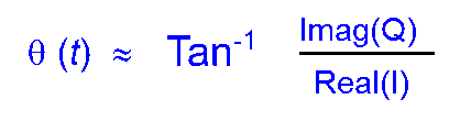
Displaying the I-Q results in terms of magnitude coordinates gives us a view of the amplitude modulation.  Displaying the I-Q results in terms of phase coordinates offers a view of the phase modulation. Taking the derivative of phase modulation yields the frequency modulation.

By adjusting the width of the low-pass filters, you can set a defined span around the center frequency where the filter width is just wide enough to pass the signal of interest, but narrow enough to filter out a lot of the noise.

 

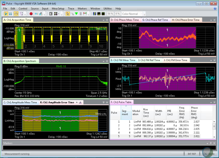
Results of digital down-conversion and processing gain on the 50-dB down RF pulse

So in short, processing gain “tunes” to the center frequency of the signal and “zooms” into the signal to analyze the modulation.

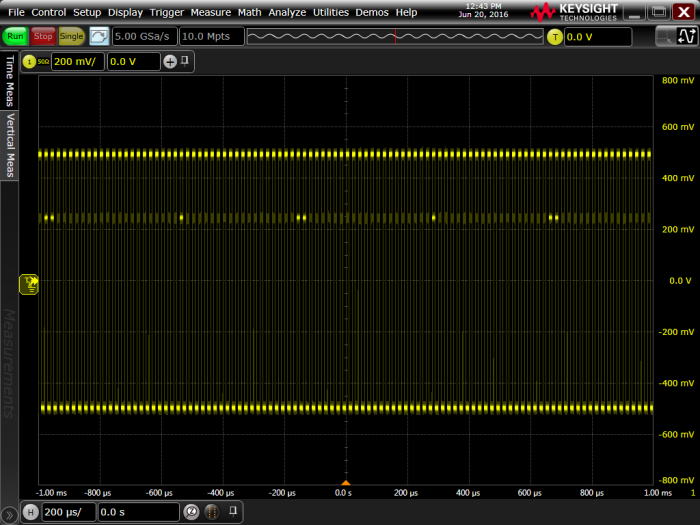
In this example, the original 8-GHz-wide measurement with the associated noise is reduced to a 500-MHz wide measurement, centered on the 3.7-GHz carrier with an instantaneous measurement bandwidth slightly wider than the width of the signal modulation.  This corresponds to an improvement in SNR as follows:

10log*(ScopeBW/Span) = 10log*(8E+09/500E+6) = 12 dB.

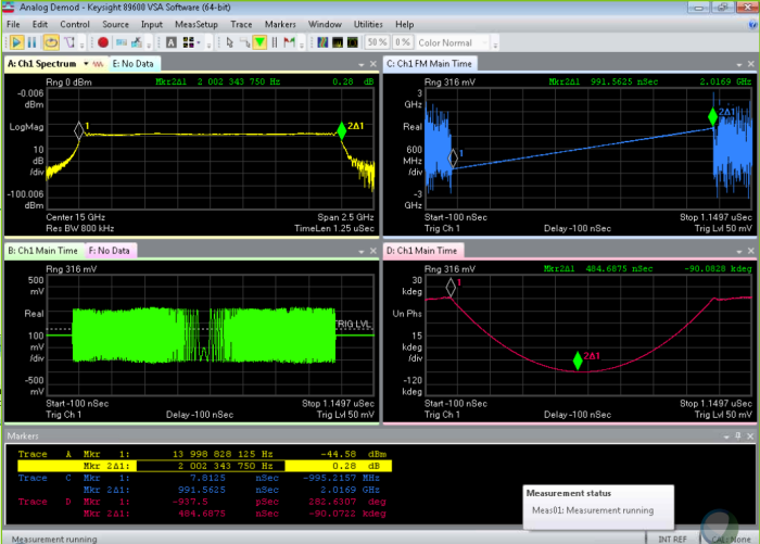
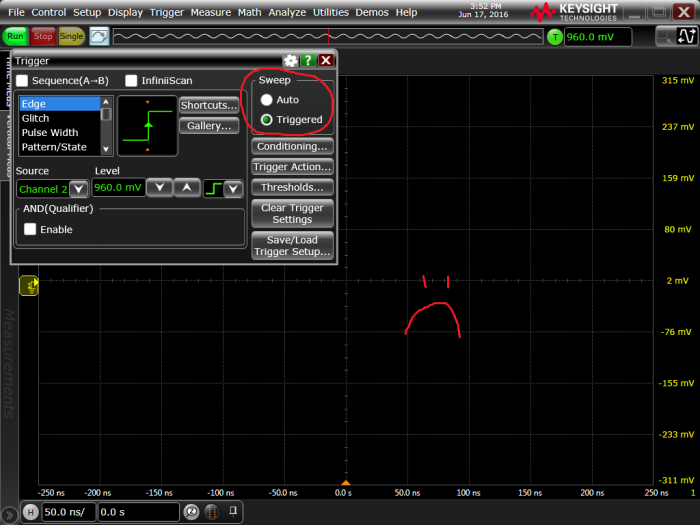
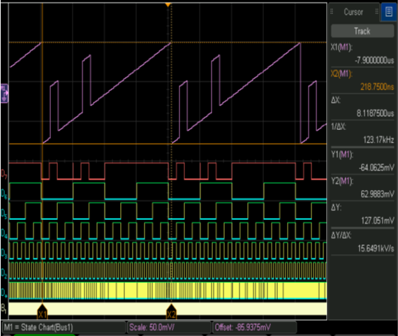
Taking advantage of this processing gain, combined with VSA software’s ability to have a log magnitude scale, and using averaging, the 50-dB down pulse is now visible, as shown in Figure 3.

Figure 3. 50-dB down pulse seen with VSA software “Center Frequency” and “Span” set to 3.7 GHz and 500 MHz

 

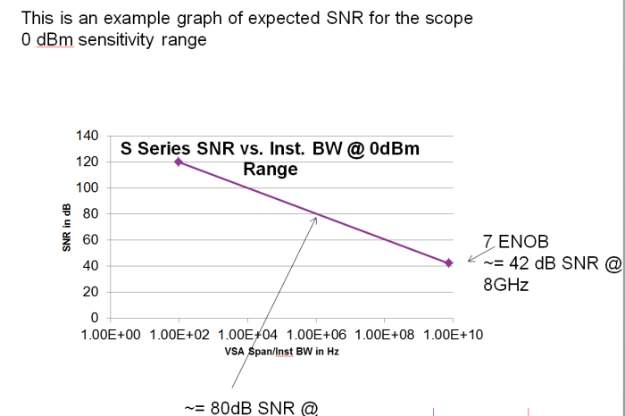
The improvement in SNR realized through narrowing down the span is depicted graphically in Figure 4.

Figure 4. Plot of SNR achievable in time view verses span adjustment in VSA software

 

 

You can draw a similar plot to see improvement in dynamic range possible when measuring narrow band signals, as shown in Figure 5.

Figure 5. Plot of dynamic range in FFT vs. resolution BW setting in VSA software

 

Here the dynamic range improvement when measuring narrowband signals in an FFT view is described as:

10log*(ScopeBW/RBW)

This does not describe the spur-free dynamic range (SFDR) or harmonic distortion characteristics of the oscilloscope response, but it does give an idea of where the noise floor will be in an FFT measurement.  As the resolution bandwidth is decreased, and the noise is divided among smaller time buckets, the noise floor drops.

This graph does not account for limitations due to various spurs, so the spur-free dynamic range (SFDR) remains limited to around 50 dB.

 

Conclusion

Through the process of digital down-conversion, the SNR of an oscilloscope measurement can be significantly improved as a function of how much that measurement can be “spanned down” from the initial DC to 3dB bandwidth of the oscilloscope.  As our example showed, a 50-dB down pulse, not even visible on a normal scope screen, can be clearly seen once processed by VSA software and then displayed in a log-magnitude scale. This approach can be very helpful to speed system validation measurements on Aerospace/Defense pulsed-RF signals. With this process, you can significantly improve measurement accuracy when evaluating the spectral, pulse envelope, frequency chirp, and phase shift characteristics of an RF pulse train.

Solutions, Solutions, Solutions!

It seems like all we hear about today in the test and measurement industry is “solutions.” Why is the word “solutions” such a popular buzz word? Well, it has a great double meaning. The first (and most obvious) definition of solution is an answer or resolution to a problem or situation. The second meaning of “solution” comes from as far back as the year 1590, and means a liquid mixture that is completely mixed (solute into solvent). When we talk about solutions, we really imply both of these definitions. One of them literally, and one of them metaphorically.

Let’s start with the literal meaning. When I say that our DDR solution kicks booty (metaphorically, not literally), what I mean is that we have a robust, industry-proven oscilloscope that will simplify the complicated task of triggering, analyzing and debugging parallel buses. If you work with DDR, you’re probably now thinking, “tell me more about this solution.” Ok, here goes:

“The Keysight Infiniium V-Series oscilloscopes also have the world’s fastest digital channels, which means you can probe at the various command signals to easily trigger on the different DDR commands such as read, write, activate, precharge and more. DDR triggering makes read and write separation easy, providing fast electrical characterization, real-time eye analysis and timing measurements. The DDR protocol decoder can decipher the DDR packets and provide a time-aligned listing window to search for specific packet information.”

So I may have copied that from our DDR webpage, but it doesn’t count as plagiarizing if it’s from my own company. And, it’s one heckuva solution because it does the job you’ll need it to do, and it does it well. If it didn’t get the job done, it wouldn’t be a solution. I also can’t just call it an oscilloscope, because it’s more than that. It’s a combination of hardware, software, and probing – it’s a whole solution.

But here’s what it comes down to, we call it a solution because it’s the answer to a lot of your DDR problems, and it’s so much more than just a piece of hardware for your bench.

Ok, I hinted above about how this could get metaphorical. The literal, chemistry definition of solution is a liquid mixture that has a fully dissolved (same root word as solution!) solute in a solvent. I don’t literally work with solutions. But when we at Keysight are combining and integrating software and hardware, we’re creating a metaphorical solution. For us to do the job 100% of the way, our software has to fully integrate (or dissolve) with our hardware. That’s what makes it a solution. It flows, it integrates, it works as one!

Ok, I also hinted that I’d get (possibly too) philosophical.  I’ll go so far as to say that we can’t really call it a solution until it’s in the hands of an engineer and being used to find solutions to bugs in their design. A solution can only be a solution when the test equipment is fully integrated (dissolved) into an engineer’s workflow and design process. The solution consists of the test tools (the solute) and the engineer’s skill and wit (the solvent). In chemistry, the solute is considered the “minor component” and the solvent is considered the “major component.” This holds true for our metaphorical solution. We can only do so much to provide the solute, the real quality of the solution is dictated by you, the solvent!

So, there’s really two main reasons we talk about solutions. 1^st, we want to convey that we can help solve your problems with a combination of tools. 2^nd, we want to partner with you to create and find the real solution, a combination of quality equipment and quality engineering.

In closing, a haiku:

Solutions, complex
Combine wit and expertise
to solve tough problems

Or more traditional English:

Roses are red
Violets are blue
I’m an engineer not a poet
solutions.

Author’s note: there may or may not have been a challenge to see how many times I could use the word “solutions” in a blog post. The answer is 32. Solutions. 33.

The Keysight S-Series Oscilloscope – The best keeps getting better!

We are moving to a new blogging platform this month. We’ll be posting to both platforms during the transition, but come check out our new location  https://community.keysight.com/community/keysight-blogs/oscilloscopes to see our future posts.

 

You may already be familiar with the Keysight S-Series oscilloscopes. They offer the best signal integrity for bandwidths up to 8 GHz, which is enabled by a set of custom technology blocks to give you:

• 4X the vertical resolution with the world’s fastest 10-bit analog to digital converter (ADC) that runs at 40 Gigasamples/sec
• Greater signal detail from a front end with 50% less noise than other portable oscilloscopes
• The ability to see your signal the way the components in your design see that signal with the highest effective number of bits (ENOB)
• Superior timing and jitter measurements thanks to timebase accuracy of 12 parts per billion
• Quick and easy analysis with more than 42 software applications
• And more! (Intrigued? Check out the data sheet)

Whether you have already purchased an S-Series oscilloscope, or are currently in the market for something in the 500 MHZ – 8 GHz range, you’ll want to check out some of the recent enhancements that make this great oscilloscope even better.  Here are just a few:

The new N7020A Power Rail Probe

The Keysight N7020A power rail probe was designed for making power integrity measurements that need mV sensitivity when measuring noise, ripple, and transients on DC power rails. Many of today’s products have tighter tolerances on their DC power rails and the N7020A power rail probe is engineered to help assure your products meet these tighter tolerances by measuring periodic and random disturbances (PARD), static and dynamic load response, programmable power rail response and similar power integrity measurements.

Key features:

• Low noise: 1:1 attenuation ratio probe for greater signal to noise ratio. Only 0.9 mVpp at 1 GHz and a setting of 2 mV/div
• Large offset range: +/-24 V offset range enables you to set your oscilloscope at maximum sensitivity and have the signal centered on the screen to view down at 1 mV/div
• Low DC loading: 50 kΩ DC input impedance will minimize load on DC power rails
• High bandwidth: 2-GHz bandwidth makes it very useful for finding high-speed transients that can have detrimental effects on clocks and digital data

When you combine the power rail probe with the signal integrity of the S-Series you can validate power distribution design specs more accurately than any other probe/scope solution.

The N7020A Power Rail probe connected to the S-Series oscilloscope

 

The new N2820A High Sensitivity Current Probe

As modern battery-powered devices and integrated circuits become more green and energy efficient, there is a growing need to make high-sensitivity, low-level current measurements to ensure the current consumption of these devices is in acceptable limits. The Keysight N2820A high-sensitivity probe is engineered to make high-dynamic-range, high-sensitivity measurements to meet these measurement challenges.

The ultra-sensitive N2820A AC/DC current probe can support measurements from 50 uA to 5 A on Keysight oscilloscopes using a make-before-break (MBB) connector, which allows you to quickly probe multiple locations on your DUT without having to solder or unsolder the leads.

It connects to two oscilloscope channels to provide simultaneous low- and high-gain views for wider dynamic range measurement. When used in combination with the Infiniium S-Series high-definition oscilloscopes this probe can deliver the ultimate high-sensitivity measurement solution.

The Keysight N2820A current probe

 

Type-C Power Delivery Decode

The Keysight N8837A Type-C Protocol Trigger and Decode software is the industry’s first oscilloscope-based USB-PD protocol decode/trigger solution.  This provides insights to USB PD engineers working on ALT mode (alternate mode) for DisplayPort, Thunderbolt 3.0, and MHL.  The S-Series are the only oscilloscopes that support hardware serial trigger on BMC signals, and allow you to quickly identify the root cause of both protocol and signal integrity issues.

Keysight Type-C Power Delivery Protocol Decode

 

MultiScope Software Application

The Keysight MultiScope software application (N8834A) provides the ability to connect up to 10 Infiniium Series oscilloscopes for 40-channels of acquisition with a tight time correlation between the scopes with very low inter-scope intrinsic jitter.  The software allows you to perform multi-lane analysis for applications such as optical networking, MIMO, DDR memory and high-speed serial standards.  These signals are presented live on a PC with the N8900A Infiniium analysis software or on the leader scope, eliminating the need for a PC.

eSPI Protocol Decode and Trigger Application

The Keysight N8835A Enhanced Serial Peripheral Interface (eSPI) was developed by Intel as a successor to its Low Pin Count (LPC) bus. So it can test and trigger on not only legacy SPI data but also embedded controller (EC), baseboard management controller (BMC) and Super-I/O with extensive triggering for all key commands and responses. This standard allows designers to use 1-bit, 2-bit, or 4-bit communications at speeds from 20 to 66 MHz.

The Keysight N8835A eSPI protocol decode

 

New Serial Data Analysis Tool Bit Error Rate Eye Contour Software

The Keysight Serial Data Analysis tool (N5394A) has been enhanced to include Bit Error Rate (BER) eye contour capability, allowing you to cut testing time from weeks to hours!  It extrapolates noise and jitter to show how an eye will close over time at various error rates.  This allows DDR4/LPDDR4 designers to make BER measurements on command and data signals. The DDR4 and LPDDR4 JEDEC spec now have new data and timing design specifications with a Bit Error Rate of <1 x 10 ^-16.   The Keysight BER contour measurement method addresses these new requirements.

Eye contours based on different bit error rates

 

New E-Band Signal Analysis Reference Solution

The Keysight N8838A E-band signal analysis solution delivers an integrated, low-cost wideband RF testing solution.  Using a high-performance oscilloscope with an external mixer and signal generator we provide an integrated down-conversion system that delivers 2.5 GHz of analysis bandwidth over the E-band frequency range of 55 to 90 GHz.

 

 

New CAN, LIN, FlexRay and CAN-FD protocol triggering and decode

The Keysight N8803C software can help electronic system designers test and debug the physical layer of automotive serial buses faster.  The CAN, LIN, FlexRay, and CAN-FD serial buses are the backbone for communication among many separate controllers, sensors, actuators, and ECUs located throughout automotive and industrial designs. These serial bus interfaces provide content-rich points for debug and test and the N8803C CAN, LIN, FlexRay, CAN-FD protocol decode is your view into these signals.

The N8803C CAN protocol decode software

 

New PAM-4 Measurement Application

The Keysight N8836A analysis software helps you quickly identify design flaws by characterizing PAM-4 signals.

Available PAM-4 real-time eye measurements include:

• Eye width, eye height, eye skew (relative) for each PAM-4 eye
• Level mean, RMS, and “thickness” for each level

PAM-4 waveform measurements include:

• Level mean, RMS, and “thickness” for each level
• Data TIE for each threshold
• Rise/Fall times for each of 6 PAM-4 transition types
• Support for CTLE, FFE, and DFE Equalization

 

 

Summary

As you can see our engineering teams have been hard at work continually adding new capabilities to our S-Series oscilloscope solution set to help you get your job done faster.

Advanced Oscilloscope Measurements and Analysis

Modern digital oscilloscopes are so capable it’s often impossible to use every feature available. But that doesn’t mean that you shouldn’t be aware of what your scope is capable of. As my father used to say, “can’t hurt, might help”. Today’s post is a preview of a webcast posted on our YouTube channel, the link can be found at the end of the article. The topic: advanced measurements and analysis using a Keysight InfiniiVision oscilloscope.

Measurements are critical to any oscilloscope user who is looking to analyze on their device under test. Whether it’s characterizing a functional design or characterizing bugs and glitches, the measurements menu is something with a lot of functionality. Additionally, our current oscilloscopes have dozens of features that are not traditionally found or expected from an oscilloscope – so we’ll review those as well.

Measurements

There are dozens of automated measurements included in Keysight InfiniiVision oscilloscopes, organized by type of measurement: voltage, time, mixed, and counting. Many of these measurements are tightly related – for example, peak-to-peak is a function of maximum and minimum, while amplitude is a function of base and top. While these may seem like identical measurements (isn’t peak-to-peak and amplitude the same thing?), our handy help text can define each one for you. Press and hold on any selected measurements and a diagram like this will appear. The webcast details each measurement and how it is made, for all four measurement types.

Math Functions

Measuring a signal as it exists is important, but what if you want to modify a signal? Examples of this might include “what would this signal pair look like after being passed through a differential amplifier?” or “what if I added a 5 MHz low pass filter to the circuit?” Our oscilloscopes have up to 27 math functions designed to manipulate signals in software to simulate many physical circuits. There are operators, transforms, filters, and visualizations.

Depending on the oscilloscope model, up to 4 of these can be displayed on screen simultaneously, and can save you significant development time. The subtract operator can be used on two analog channels to display the differential output, while the low pass filter can be used to emulate a 5 MHz filter on your signal, all without having to develop anything in hardware! The image below shows the simulated output of a signal through a 5 MHz low pass filter.

Analysis Tools

Some of the most powerful tools in the oscilloscope live in the analysis menu. Things like histograms, mask testing, eye diagrams, and frequency counters come as options in many models. While advanced triggers and measurements can help with isolating and characterizing a signal, the analysis tools in the oscilloscope are part of the final step of troubleshooting, which is root cause analysis. As an example, histograms can be used to visualize the distribution of measurements or waveforms. In this screenshot, we are looking at the distribution of period measurements over the course of a few minutes on a clock signal with some timing jitter. The shape of the histogram tells us the signal has periodic jitter due to its bimodal shape. Learn more about jitter here!

Summary

After exploring each measurement, math function, and analysis tool, we take some time at the end of the webcast to show you real world examples of how all these functions can be combined to solve problems. The core purpose of an oscilloscope is to help you identify, isolate, and determine the root cause of physical layer issues in your design, and we sincerely believe that our scopes can help you do that easier and faster than anything out there! Check out the Advanced Oscilloscope Measurements and Analysis webcast video .

Thanks and happy watching!

High Bandwidth Oscilloscope + Analysis Software = Powerful, Wideband RF Measurement Suite

A change is coming in the tools for measurements in both pulsed RF aerospace/defense and I/Q vector-modulated communications application. Whether for multi-channel analysis or for wider analysis bandwidth, high-bandwidth oscilloscopes are taking the place of traditional spectrum and signal analyzers. That’s because they can handle signals with spectral content beyond 1 or 2 GHz. These signals are being created to support the higher resolution requirements in radar systems and move the vast amounts of information in new communications systems.

So how do you create a powerful, wideband RF measurement suite? By coupling a high-bandwidth real-time oscilloscope with RF analysis software. Once you’ve married the two, you achieve a number of enhancements:

• Noise reduction through digital down-conversion
• A wide range of vertical scaling options, including linear and log magnitude
• Key RF measurements including occupied bandwidth (OBW) and power spectral density (PSD)
• Vector demodulation options for communications formats like QAM16
• Analog demodulation options including AM, FM and PM
• Set-up of segmented memory capture
• Statistical pulse analysis

 
Pulse amplitude, frequency, phase, and FFT measurements

For radar and electronic warfare applications, it’s helpful to perform a variety of measurements on many pulses. This includes things like amplitude variation, frequency, and phase shift across pulses, and a view of the spectrum of signals. For applications such as aircraft warning receivers, you also want the capability to measure time difference and phase difference between pulses associated with the capture of a wave front by multiple antennas on an aircraft. Let’s consider some of these measurements.

In the simplest case, you can measure the basic pulse amplitude, frequency shift, and phase shift across the measured RF pulse. The RF pulse train is sampled by the oscilloscope and then digitally down-converted to reduce noise and allow further signal processing.

For example, in Figure 1, a 15-GHz carrier, 2-GHz-wide linear FM chirped RF pulse signal is shown after vector signal analysis (VSA) processing. Here’s what the image shows:

• 2 GHz-wide spectral content of the signal (upper left);
• Real part of the down-converted I/Q data (lower left);
• 2-GHz-wide linear FM frequency chirp seen across the RF pulse (upper right);
• parabolic phase shift seen across the RF pulse (lower right).

These measurements are taken in the “Vector” measurement mode.

Basic vector mode analysis of FFT, real part of I/Q, FM chirp, and phase shift across pulse seen

 

Single channel, segmented memory capture, statistical RF pulse analysis

The next level of analysis requires a shift into “Pulse Analysis” mode. Here we use multiple oscilloscope channels to capture RF pulse signals into segments of oscilloscope memory. These are digitally down-converted into baseband I/Q signals, and then evaluated for single and multiple channel pulse analysis. For single-channel measurement, you can make three comparisons:

• the linear FM frequency chirp to an ideal, best-fit linear FM chirp signal;
• the phase shift across a pulse to a best-fit parabolic phase shift profile;
• the amplitude of the pulse envelope to a best fit ideal straight-line best fit reference.

In Figure 2, you’ll see these comparisons being made between measured to reference, and then the “error” between the measured and reference is expanded in vertical scale for a close view.

A pulse table also displays RF pulse parameters, including an RMS error calculation between the measured frequency or phase across the pulse, compared to a best-fit reference signal. It’s also possible to show statistics for the measurements over all the pulses.

Single-channel spectrum, amplitude, phase, and frequency measurements vs. best-fit reference signals

 

Dual-channel delta pulse amplitude, frequency, and time-delay measurements

You can also make “two-channel delta” measurements, as shown in Figure 3. These measurements are becoming increasingly important in applications such as aircraft warning receiver testing, where multiple signals are being captured from multiple antennas. The time delay and frequency difference of arrival between wave fronts must be measured for angle-of-arrival calculations.

Notice in this example a 1 nsec time delay being measured between two RF pulses. You’ll also see a 0.2-dB difference in amplitude and a 16-kHz difference in frequency, on average.

Pulse analysis is also performed on three of ten captured pulses that are being placed into oscilloscope memory segments. The parabolic phase shift across pulses (lower left), the linear FM chirp frequency shift across pulses (middle right), and the pulse envelope of pulses (upper left) are superimposed for signals coming into two oscilloscope channels. As in the previous example, each scope-channel measured signal can have the measured, reference, and error signal calculations made. Finally, the FFT spectral content for both scope-channel captures of the two pulse trains (center left) is also shown.

Two-channel measurements of RF pulse characteristics including time, amplitude, and frequency difference between two channels

 

Cross-correlation between pulses for precise time-delay measurements between RF pulses

In the aircraft warning receiver example mentioned previously, you can determine very precise measurements of time delay between RF pulses captured on different antennas on an aircraft by using a cross-correlation measurement between pulses. In Figure 4, a 50-psec time difference of arrival (TDOA) is being measured between two RF pulses captured on two scope input channels. Here pulses have a 10-GHz carrier, 100-MHz-wide linear FM chirp modulation, and a 1-usec width. In this measurement, you can first remove the channel-to-channel skew between oscilloscope channels, including cable delays at the temperature measurements will be taken, through de-embedding. Then a measurement can be made to see the actual time shift between the captured signals. Measurements show a mean delay of 50 psec, with a peak-to-peak variation in delay between 47 psec and 53 psec.

Two-channel cross-correlation measurement for precise time delay between pulses

 

Math function used to measure phase shift between two RF pulses

The difference in phase between two RF pulses is also critical in a variety of radar/EW/warning receiver-oriented applications. Through the use of math functions, the measured phase across one pulse can be subtracted from the measured phase across a second pulse, measured on two oscilloscope input channels. We can measure the same two linear FM chirp signals from the last example to view the phase shift between the two pulse trains by comparing related pulses. Again this might be seen from two antennas on an aircraft. The time shift has now been set to zero on an arbitrary waveform generator, but a 25-degree phase shift is being introduced between the two signals. A capture shown in Figure 5, top center trace C, and related blue marker 1, show this 25-degree phase shift in a mean measurement in lower right Trace D, as well as only a 0.8-degree standard deviation and a 0.7 variance.  These are average values over the width of the pulses.

Two-channel phase difference measurement between two RF pulses

 

Summary

More radar/EW/warning receiver applications are driving toward wider modulation bandwidths to increase range and angle-of-arrival precision capability in related systems. At times, this extends beyond 1-GHz modulation bandwidths. Designers increasingly use wideband oscilloscopes as RF receivers to evaluate related wideband signals when validating their hardware prototypes. Although scope measurements directly are of interest, it’s often advantageous to use analysis software to digitally down-convert captured wideband signals to reduce noise and allow more in-depth analysis of baseband I/Q signals. By combining a wideband scope and VSA software with appropriate techniques, you can readily make angle-of-arrival calculations for a variety of systems.

Understanding Oscilloscope Trigger System Basics & Why You Should Care

You sit down at your lab bench to debug some funny behavior in a 10 MHz clock.  You fire up your oscilloscope, get your probing in place and hit the almighty Auto Scale button, after which you’re presented with something like this:

Figure 1: 10 MHz square wave after Auto Scale

and then it strikes you; there are ten million clock cycles occurring every second!  How in the world is the scope able to accurately display such a clean representation of your signal?  How is it that the middle of the rising edge of your clock is perfectly aligned at center screen?  The answer is the trigger system.

The trigger system is both one of the most commonly-used and least-understood sub-systems in real-time oscilloscopes.  In this article I’m going to pull back the curtain just a bit and explain what the trigger system does, how it works and why you should care.

 

What It Does

The sole responsibility of the trigger system is to tell the rest of the oscilloscope what data to care about.  It decides when the acquisition system begins acquiring, which means that by default it decides what is displayed on screen and what data is available to make measurements on.  It can make these decisions with a very simple set of conditions or very complex conditions, based on user input.  Let’s consider the example above; a 10 MHz square wave.  The reason the signal in the image above looks so clear and well-positioned on-screen is that the trigger is set up, appropriately, to look for a rising edge on Channel 1:

Figure 2: Trigger setup as configured by Auto Scale

Remember that to start we used Auto Scale, which was kind enough to pick an appropriate trigger source and threshold based on our input signal.  But what would our signal look like without an appropriate trigger configuration?  I’m glad you asked:

Figure 3: 10 MHz square wave, auto-triggered. Infinite-persistence is enabled on Channel 1 to better illustrate what’s going on

In Figure 3 above I have changed the trigger condition to look for an edge on Channel 2 (which has no signal connected at the moment).  The auto-trigger feature, which we can see is enabled in the “Sweep” section of the trigger configuration dialog, is automagically kicking off acquisitions on a regular time interval giving us a smear of yellow signal trace across the screen.  The signal itself appears to be clearly visible in this image, superimposed over the “smeared” signal trace, unfortunately however this is just an artifact of the screen shot; that’s where the signal happened to line up at the instant I took the screen capture.  In practice, auto-triggered acquisitions aren’t good for much of anything other than to determine the relevant DC parameters to use in setting up your trigger condition.  Note that if the auto-trigger feature is disabled, without an appropriate trigger configuration the oscilloscope simply won’t acquire:

Figure 4: Disabling the auto-trigger feature without an appropriate trigger configuration means the oscilloscope won’t acquire at all.

The trigger system will always place the trigger point (the instant at which all conditions present in the trigger configuration are met) at t = 0.0 s on screen.    Later on, we’ll see how using advanced trigger configurations can help capture infrequent and hard to find events, in addition to the simple rising-edge trigger we’ve seen so far.

 

How It Works

Most real-time oscilloscopes have an “analog” trigger system.  This system is actually a mishmash of analog circuitry and digital counters but it relies on input from analog comparators fed from the scope pre-amp.  Some oscilloscopes now feature a “digital” trigger, meaning that the trigger system is entirely digital and is fed with integer data from the ADC output.  Both types of systems perform the same function; evaluating whether or not all of the configured trigger conditions are met at a given moment in time.  Because fully digital trigger systems are fairly rare, we’ll focus on analog trigger systems.

Figure 5: Generic four-channel DSO front-ends and trigger system

Figure 5 above shows a generic representation of the parts of a four-channel DSO (digital-storage oscilloscope) that we’re concerned with; the analog channel front-ends and the trigger system.  The trigger system takes inputs from comparators on all of the analog channels and provides a single output.  For convenience, let’s focus on a simplified diagram with only one analog channel:

Figure 6: Generic DSO front-end and trigger system

Figure 6 is a simplified, one-channel view of the same systems depicted in Figure 5.  When a signal is connected to the channel input it goes through a series of transformations before it ends up on-screen:

• First, the signal is scaled appropriately and offset if necessary by the pre-amp. The pre-amp output is sent to the ADC to be digitized.

• Trigger comparators observe the output of the preamp and fire if it exceeds the threshold they have been set to. This threshold is set based on user input, or by helper routines like the almighty Auto Scale.

• The trigger system observes all of the trigger comparator outputs in the system and combines them in such a way as to monitor for a given set of conditions. These conditions can be very straight-forward (IE: rising-edge on channel one) or quite complex (IE: pulse-width greater-than 2.4 ns on channel 3, followed by a pattern of channel one high, channel two low and channel four low, held for a duration of greater-than 30.0 ns and less than 50.0 ns).

• When the trigger system sees that all of the conditions are met for the specified trigger, it sends a pulse on its output. We call this signal “System Trigger” or “SysTrig” for short.  SysTrig is monitored by the acquisition system as well as a special sub-system known as the “time-base interpolator”.

• When the acquisition system sees a pulse on SysTrig, it begins to digitize, process, store, measure and finally display data. We refer to this entire process in general as “acquisition”.

• Before the acquisition data (the waveform) which is now stored in memory can be displayed on-screen, we need to know how to orient it horizontally; this is where the time-base interpolator comes in. The interpolator monitors SysTrig, just like the acquisition system.  When it goes high, it’s the interpolator’s job to figure out what address in waveform memory matches up with the instant the trigger occurs.  It communicates this information to the acquisition system and voila, the result is the desired waveform on-screen, with the trigger point placed perfectly at t = 0.0 s!

 

Why You Should Care

Although some of you may find the inner workings of oscilloscope sub-systems interesting, it’s fair to say that most folks couldn’t care less.  If you are one of those folks and you just skipped the entire “How It Works” section above, no sweat, there will not be a quiz at the end!  The bottom line is that you should care about the trigger system and take the time to understand it because it can help you debug difficult issues and save you quite a bit of time and frustration.

Using an oscilloscope in a basic way, that is to say, pushing the Default Setup and Auto Scale buttons can tell us a little bit about our signal and is a quick and convenient way to get started.  However, if you’re interested in capturing an infrequent event, as is often the case when debugging common issues like runts, glitches and setup & hold violations, the trigger system is a powerful tool.

 

Advanced Trigger Modes

In addition to edge trigger mode discussed at the beginning of this article, most real-time oscilloscopes have a number of advanced trigger modes designed to detect common problems.  When used in conjunction with “Triggered” sweep (aka, auto-trigger disabled) these modes will ensure that only the behavior you’re looking for is acquired and displayed.  As an example, let’s look for a runt in a square wave.  We connect our signal, use our trusty Auto Scale button and all we see is a square wave, no runt in sight!

Figure 7: Looking for runts in all the wrong places…

Figure 7 shows us that although we suspect a runt is present in our signal, finding it with edge trigger will prove difficult.  Maybe we’ll be able to see it if we zoom out a bit?

Figure 8: Looking for a runt with edge trigger, zoomed out horizontally

As shown in Figure 8, by zooming out horizontally we can tell that there’s something fishy going on, but it’s not entirely clear what.  Now, let’s use runt trigger mode on our Infiniium S-Series oscilloscope and see what we can find:

Figure 9: Runt trigger mode setup on an Infiniium S-Series oscilloscope

 

Figure 10: Looking for a runt with runt trigger mode

There’s our runt!  The waveform in Figure 10 is clear and steady and the event we’re interested in, our elusive runt, is right at t = 0.0 s!  This is the value of learning the trigger system on your scope, it will allow you to find the events you’re interested in, and only the events you’re interested in, very quickly.  Although this example focused on finding a runt, the same sort of example can be demonstrated with glitches, setup & hold violations, specific data across multiple channels, data patterns relative to clock edges, edge transition times, etc. using the appropriate trigger mode.

 

Advanced Trigger Features

In addition to advanced trigger modes like runt mode discussed above, many oscilloscopes have features that can be used in conjunction with trigger modes to further refine what we want the oscilloscope to show and to instruct the scope to automatically take actions when a trigger occurs.

Figure 11: Trigger Conditioning dialog on an Infiniium S-Series oscilloscope

Figure 12: Trigger Actions available on an Infiniium S-Series oscilloscope

Figure 11 above shows some common options for trigger conditioning, while Figure 12 shows some of the things we can configure the oscilloscope to do for us automagically when a trigger occurs.  My personal favorite is the “Email on Trigger” feature.  If you have a really infrequent event, no problem; set up your trigger and leave for the weekend.  Come back, open up your email and find all the data you need!

Thanks for reading!  If you have specific questions regarding triggering or challenges triggering on a specific event let us know in the comments!

Inventing the MSO

A look into the history of the mixed-signal oscilloscope

1996 was a year to remember, it brought us the Macarena, the Nintendo 64, and the first Motorola flip phone.  But, also making its debut that year was the HP54645A mixed signal oscilloscope.  Today mixed signal oscilloscopes (MSOs) are an industry standard, but this was new and exciting technology 20 years ago.  Here’s an excerpt from the HP journal from April 1997:

“This entirely new product category combines elements of oscilloscopes and logic analyzers, but unlike previous combination products, these are “oscilloscope first” and logic analysis is the add-on.”

At this point in the tech industry, microcontrollers dominated the landscape. Gone were the 1980s and the days of microprocessors and their dozens of parallel signal lines, in was the 8-bit or 16-bit microcontroller. As the need to test dozens (or hundreds) of channels decreased, the thriving logic analyzer industry began to shift in favor of oscilloscopes.  As a result, Hewlett Packard released the 54620A; a 16-channel timing-only logic analyzer built into a 54645A oscilloscope frame. This was a big hit for engineers who only needed simple timing analysis from a logic analyzer and liked the simplicity and responsiveness of oscilloscopes.

These tools were all coming out of Hewlett Packard’s famed “Colorado Springs” division, which focused heavily on logic and protocol products. In hindsight it’s clear that the shift from a logic analyzer-focused landscape to an oscilloscope-focused landscape was inevitable.  But, when the project funding decisions had to be made the logic analyzer was king.

A few R&D engineers, however, saw it coming.  They strategized amongst themselves to get a new oscilloscope project underway.  However, they knew it was going to be a hard fought battle. Following the old adage “if you can’t beat them, join them,” the engineers proposed a new project combining the oscilloscope and the logic analyzer into one frame. The thought was that if an oscilloscope project wouldn’t get funding, then surely integrating a logic analyzer into the scope would do the trick. Below is a picture of Bob Witte’s (RW) original notes from the 1993 meeting in which the MSO was conceived. (Follow Bob Witte on Twitter: @BobWEngr) This product was internally code named the “Logic Badger,” stemming from the 54620A oscilloscope’s “Badger” code name and the 54645A’s “Logic Bud” code name.

One thing led to another, and the 54620A and the 54645A were combined into the paradigm shifting 54645D. A new class of instrument was introduced into the world: the mixed signal oscilloscope. For the first time ever, engineers could view their system’s timing logic and a signal’s parametric characteristics in a single acquisition using the two analog oscilloscope channels and eight logic channels.

From its somewhat humble beginnings, the MSO has become an industry standard tool globally, with some estimating that up to 30% of new oscilloscopes worldwide are MSOs. Logic analyzers are also still sold today and are an invaluable tool for electrical engineers thanks to their advanced triggering capabilities, deep protocol analysis engines, and state mode analysis. If you’re debugging FPGAs, DDR memory systems, or other high-channel-count projects you’ll want to consider using a logic analyzer. However, mixed signal oscilloscopes dominate today’s bench for their ability to quickly and easily trigger and decode serial protocols.

Finally, it’s worth noting that the Hewlett Packard division is still alive and strong in its current form here at Keysight Colorado Springs. In fact, many of the same engineers from the very first MSO project are still here working on today’s (and tomorrow’s) MSOs.

To learn more about how the digital channels on an oscilloscope work, check out this 2-Minute Guru video on the Keysight Oscilloscopes YouTube channel.

Learn more about MSOs or view the mixed signal oscilloscopes available today from Keysight Technologies at Keysight.com.

Why Would you Want a Mixed Signal Oscilloscope?

As an oscilloscope user you understand the importance of analyzing analog signals in a digital circuit. However, many users are missing out on one of the most powerful features of today’s oscilloscopes: the mixed signal oscilloscope (MSO). An MSO adds up to 16 digital channels to your 4 analog channel oscilloscope. This greatly expands the types of analysis that can be performed by this versatile engineering tool. Digital signals can be a simple chip select, or a communication bus. The ability to monitor these digital signals is often critical to properly analyze system operation.

Debugging a mixed signal design can be a difficult and somewhat daunting task to the engineer who is armed with a 4-channel oscilloscope since you often need to capture more than four signals. An mixed signal oscilloscope provides that capability, with the ability to examine the state of up to 20 signals all on the same timescale, while using the familiar controls of a basic oscilloscope.

When needed, MSO digital channels provide just enough logic analysis for users whose home base is an oscilloscope. MSO digital channels serve as an extension to the oscilloscope capabilities and can provide valuable insight into the operation of your design.

Correlation of input/output of ADC/DAC is simple and straightforward. An MSO adds some very powerful and useful tools for analyzing a digital bus. In this one simple view we can see the state of the analog signal, the state of each of the digital signals, the hex representation of this digital bus, and I still have all of the measurements available on the oscilloscope to evaluate the signal quality. The controls and measurements are all still based on the oscilloscope operation, making it very easy to navigate and control.

At the same time the MSO provides the means to help analyze your digital bus. The grouping of digital signals to create a “bus” with easy-to-read hex values can be used in decoding the signals, or for triggering on specific addresses or values.

MSOs and logic analyzers have fundamental architectural differences in how they acquire and display signals. MSOs exclusively use asynchronous sampling, just like an oscilloscope. For many users, this makes setting up an acquisition on digital channels simpler, because it feels like a scope.

By applying some additional logic to the digital bus you can create a visualization of the bus operation. By using one of the signals as a clock, the MSO can chart the bus “state” to display a logical representation of the digital data.

Displaying an analog equivalent of the data that is being transferred across the bus can quickly identify errors in the digital data.

 

Low-Speed Serial Bus Support

Today’s designs incorporate digital communications between components and systems by using high- and low-speed serial digital communication, and microprocessor buses. Serial buses like I²C and SPI are frequently used for chip-to-chip communication, but cannot replace parallel buses for all applications. But here again, oscilloscopes add powerful troubleshooting capability by providing just enough protocol analysis.

A key difference between logic analyzers and MSOs is the latter’s ability to trigger on and decode serial buses. Low-speed serial buses are ubiquitous in electronic designs because of their ease and low cost of implementation. In fact, it is hard to find a design that does not include at least one I2C or SPI bus, or USB.

Mixed signal oscilloscopes excel at debug that includes low-speed serial buses. All good MSOs come with both triggering and decode options for serial buses. However, logic analyzers have not incorporated similar triggering and decode technology. Without protocol triggering, it’s impossible to set up the oscilloscope to trigger on specific packets. For example, you can set the MSO to trigger when an I2C read to a certain address with a certain data value happens. Alternatively, you can trigger on a certain SPI data packet or at the start of USB enumeration.

Since the blending of analog and digital information is so prevalent, oscilloscope users can take advantage of the ability of current MSOs to improve their troubleshooting capabilities and simplify their mixed-signal design debugging.

Keysight oscilloscopes have the added benefit that most existing DSOs (Digital Storage Oscilloscope) can be easily upgraded to add MSO capabilities.

If you are reading this before September 30^th 2016 and you are in the market for a new oscilloscope, you can take advantage of Keysight’s MSO promotion. You can add MSO capabilities to a new 3000T, 4000, and 6000 X-Series oscilloscope for no additional charge!

Learn more about MSOs!

Insider Tips for Using an Oscilloscope with Touch

Author: Chris Felder

As one of the Keysight R&D engineers who developed Project Echo, the touch screen and interface for Keysight InfiniiVision oscilloscopes introduced on the 4000 X-Series in 2012, I know these oscilloscopes from the inside out; literally. Here are a few creative shortcuts we have built into the oscilloscope interface to help you get more out of the scope.

As Keysight was designing the first touch interface, which is used on the Keysight 3000T, 4000-X, and 6000-X Series scopes today, we conducted extensive usability testing to ensure the touch screen and interface design enhanced the existing interface and the scope could be entirely driven using the touch screen. While touch can provide many benefits, we also wanted to be sure that it did not impair the usability for those not using the touch feature. Even if you prefer to drive the scope using the front panel keys and knobs, using touch in minor ways may greatly accelerate your tasks.

Let’s start with the “main menu” button in the upper left corner.

All of the oscilloscope’s menus and dialogs are accessible through this menu.  There are some handy shortcuts along the left side, and you can manipulate several feature states directly through this menu (channels, cursors, measurements, etc.).  The Applications menu gives a list of your licensed and installed oscilloscope applications, but also lists unlicensed applications – handy if you’d like to explore and read about all the capabilities built into your scope.

From the main menu, we move on to the status area along the top of the graticule; this area hold lots of readouts that show the state of the oscilloscope, and all of them are touchable.  Touch the scale or delay values in the Horizontal grouping, for instance, and you’ll get this handy popup:

 

From here, you can step the values using buttons, or touch the values once more to get a numerical keypad for direct entry.  If you want to change other timebase settings, you can press the gray ‘H’ button in the status area for a quick shortcut to the Horizontal softkey menu.

 

In some areas, we’ve added more significant shortcuts for the most common tasks.  Touch the trigger status indicator, for example, and you immediately toggle from Auto mode to Normal mode, and vice-versa:

 

The sidebar along the right side of the screen is another area we’ve really optimized for touch.  Any dialog box with a series of dots in the upper left (what we call a “gripper”) can be repositioned by dragging it from the title bar area; the same is true of sidebar tabs.  Any tab can be grabbed using the grippers, undocked, and positioned anywhere you like.  You can even re-dock the tab in a half-height mode, allowing you to see two tabs at once:

Like the status area, sidebar tabs are filled with touch shortcuts.  You can touch the analog channel input information in the Summary tab to quickly perform a slew of front end and probe configuration settings:

Titles in the sidebar tab look a bit like buttons for a reason – they all have handy shortcut menus when you touch them.  Touching the title in the Cursors sidebar, for example, lets you directly change mode and source settings without needing to travel to the Cursors Menu:

 

 

 

 

In the Measurements tab, you can touch individual installed measurements to track, clear, or reset them:

 

 

The softkey menu area along the bottom of the screen frequently includes readouts for status items related to the current menu, and…you guessed it…they’re all touchable! If you have the WaveGen (waveform generator) option enabled on your scope, the Waveform Generator Menu contains a particularly handy shortcut; if you touch the “Gen Out” area, you get a comprehensive control stack for the selected WaveGen, from which you can change a variety of settings without bouncing between multiple softkey menus:

Like all dialog boxes, this dialog can be re-positioned by dragging it within its title bar area.  You can also use the blue Menu button to configure dialog boxes to use a transparent background.  Now you can position and configure dialog boxes and sidebar tabs as you wish!

We strive to follow the rule, “everything is touchable” and we’re constantly adding new shortcuts and convenience menus with every software release.  We always welcome your suggestions and feedback – comment here to let us know what we can do to make your oscilloscope experience more efficient.

Welcome to Scope Month!

Welcome to Keysight’s inaugural Scope Month – an entire month focused on oscilloscope measurement tips, new content and oscilloscope giveaways! Join us throughout March for great oscilloscope resources and activities, including:

• New Oscilloscope Learning Center
  • You already have the expertise and ability to perform your job at a high level. Keysight wants to help by offering you the tools and information you need. As part of this, we are launching the Oscilloscope Learning Center where you can access a wide variety of information – from basic to advanced. Find application notes, measurement tips, videos, articles, and webcasts all in one location.
  • Content will be updated often so check back for the latest information and answers to your questions.
  • www.oscilloscopelearningcenter.com
• Scope-a-Day Giveaway –Over $500,000 in daily oscilloscope giveaways!
  •  This is the largest scope giveaway we have ever done, with over $500,000 USD in oscilloscopes being given away during Scope Month!
  • We will be giving away one MSOX3104T oscilloscope per day during Scope Month.
  • We will also be compiling the entries each week during Scope Month and picking a weekly winner via a live video stream. These weekly winners will be awarded an MSOX4104A oscilloscope.
  • Submit your entry and view the legal terms and conditions at www.scopemonth.com. And don’t forget to enter every day.
• “Test to Impress” Contest – win a fully-loaded 6 GHz scope, valued at over $70,000!
  • Throughout Scope Month, you can submit a 1-2 minute video describing how you have used (or would use) InfiniiVision oscilloscopes to impress; by solving a measurement challenge, working on a cool application, etc.
  • During the first two weeks of April, Keysight will post these videos and you,with the rest of the engineering community, will be able to vote on your favorite submissions to decide the winner (announced April 15^th).
  • The winner will receive a 6 GHz 6000 X-Series oscilloscope, four N2752A InfiniiMode 6 GHz differential probes, and a 6000X application bundle – valued at over $70,000!
  • Submit your Test to Impress entry . You can also see the legal guidelines and eligible countries.
• 2-Minute Guru Video Series
  • In addition to the Oscilloscope Learning Center, we are creating a video series called the “2-Minute Guru” which will provide information regarding scope basics. These will be launched throughout Scope Month and will continue beyond the month as well. Check the blog frequently to be notified when the next episode is available.
• New Limited-Time offer – Get an MSO for the Price of a DSO!
  • Until September 30^th, 2016, you can purchase an MSO model of select Keysight InfiniiVision Series oscilloscopes for the price of a DSO.
  • Visit Keysight MSO offer for more information.
• Webcast Series
  • Throughout 2016, Keysight will be hosting a series of oscilloscope and measurement webcasts. You can view and sign up for the entire series, or watch previously recorded webcasts on your schedule by scrolling to the bottom of that page.
• “Will It” Videos
  • InfiniiVision oscilloscopes are known for their instrument integration – offering you more value with your purchase by embedding other instrument functionality into the oscilloscope. Our marketing team has taken this one step further and has asked our R&D team to add several new features to our scopes. The question now is “will the oscilloscope be able to perform the tasks?” Watch these humorous videos every Friday during Scope Month.

And much, much more…

 

We hope you enjoy this exciting event, are able to join in some of the fun and also learn some new things as well. Stay up-to-date on this blog and our social media pages to see what else we have coming!